
Processing The Flame & Horsehead
1 December 2022Lots of intermittent clear skies and cloud over the past week or so, but I managed to pull together some really nice shots of The Flame and Horsehead Nebulae over three nights. Quite a few of the frames had significant amounts of cloud, so I chose not to stack them and I ended up with about three hours of good data.

So having gone through my shooting workflow in the previous post, here’s a rough processing workflow based on this image.
YouTube has been an amazing learning resource, in particular for processing and editing. I’ve learned various approaches to the same aim – to pull out the maximum amount of image information from the data that is contained in the image. But basically it falls into these categories:
STACKING
There are various stacking programs, but Deep Sky Stacker (DSS) is probably the most used software and it’s free. Stacking multiple images does two things:
1) Increases the total amount of exposure. So, 40x15sec stacked exposures is the same as opening the shutter for 10 minutes.
2) Reduces the amount of noise (graininess etc) resulting from using high ISO and slow shutter speeds.
It’s all about signal to noise ratio. Signal is the information you want – the stars, the nebulosity etc. This is in the same place in each frame and the stacking software lines up the frames using these. The signal is also further enhanced by the stacking, and the more total integration you have the more detail can be drawn out. Many hours of integrated exposure are ideal.
Noise is the stuff you don’t want – and importantly noise due to long exposure etc is random and does not appear in the same place in each frame. So this is averaged out over the individual frames in stacking, reducing the noise in the stacked image.
However, some unwanted signal can occur within the camera from dead pixels, hot pixels and general sensor issues in the camera. These will not be random, so a series of calibration frames are also taken to identify these, so that DSS can remove them.
The image that DSS presents you with after stacking (which may have taken many hours to do) is amazingly underwhelming! Usually just grey with various sized white blobs. But this contains all the information that needs to be stretched.

master image for processing
‘STRETCHING’
This is the key to Astro processing and can be done in Photoshop (or other programmes – Pixinsight is specifically designed for Astro, but is very different to PS apparently). Stretching is pulling out the maximum amount of detail from the stacked image (the data) whilst controlling the exposure and noise levels as much as possible.
When you first look at the Histogram in PS, there will be just a thin slither to the left – that’s because the image is mostly black/grey. By careful and repeated adjustment of Levels and Curves the details begins to appear and the histogram becomes ‘fatter’ and more balanced. These stretching adjustments are applied gradually (not all at once) ensuring the blacks are not crushed and the whites are not blown.

The DSS image first opened in Photoshop 
Some initial stretching using
Layers and Curves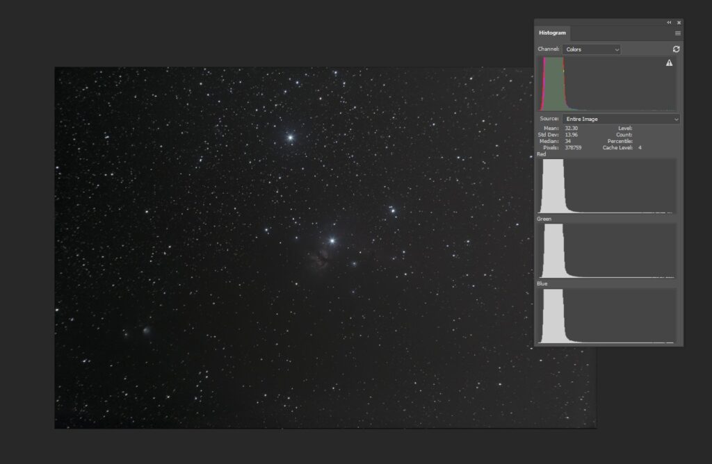
And after another Curves stetch
By the end of this initial Stretching process, the Flame is clearly visible and the Horsehead is just about starting to show through
OTHER TECHNIQUES
You can get pretty good results with just careful use of Levels and Curves and with a bit of Sharpening, Noise Reduction and Colour Saturation tweaking too. But there are other little secrets too.
Background Gradient
As the data is stretched, more unwanted gradient in the sky becomes evident. Much of it is caused by light pollution (ie lighter at the bottom, darker at the top.
In the case of this image, it has been rotated so the gradient is lighter on the left (as you can see in the last edit above).
Gradient can be reduced fairly early in the process by copying the image, filtering out the stars, smoothing it using blur and dust and scratch removal, then applying the image back to the original. There’s also a plug-in software (not free) called Gradient Xterminator.

The result after reducing the gradient
One the gradient has been reduced, the histogram shows that the dynamic range has reduced again (we’ve removed a large part of the mid-tone), so some more stretching follows
Star Removal/Separation
This is a game changer! As you stretch the data, the stars become brighter until the point that they are over-exposed and detract from subject of the image. So, by ‘saving’ and removing the stars only from the image when they are still nicely exposed, you can process the sky and the DSOs then add the stars again as another layer. This gives you separate control over the main image and the stars. Many astrophotographers reduce the brightness and even the size of the stars to better enhance the subjects of the image.
There is another free programme, StarNetv2GUI which deals with the star removal. So once I’ve reached the point where I don’t want the stars to get any brighter, I save image (as a large tiff file) to run through StarNet. The resulting image is then opened in Photoshop (along with the existing work) and doing a subtraction of the the complete image and the starless one, I get a nice Stars Only lay, which can be overlaid on the background.

The Starless Image 
The Stars Only Image 
Starless with some more processing and colour pulled out 
The Stars replaced
At this stage, that’s pretty much all I do in Photoshop. I’ll save the image (as a tiff file again) and import into Lightroom for some final sharpening, noise reduction, cropping and colour tweaking . Of course you could do much the same in Photoshop’s Adobe Camera Raw filter, but I use LR so much in my other work that I feel more familiar with general editing in it. Plus I can also easily duplicate the images, synchronise the edits etc then save in various file-sizes with and without watermarks, some cropped square and so on. I’ve also found that images destined for Social Media need to be less black, so I’ll make some edits and save for Facebook posts etc.

